Visual tutorials

These examples run the current Rustures wheel on deterministic synthetic signals. The dark dashed lines are the known changes used to generate each signal; the red lines are the changes predicted by Rustures. Returned breakpoint lists also contain the terminal sample, even though it is not drawn as a change.

Examples, not benchmarks

Parameters were selected to make each algorithm's behavior easy to inspect. These figures demonstrate API use and output semantics; see Performance for controlled timing measurements.

One signal, five search strategies

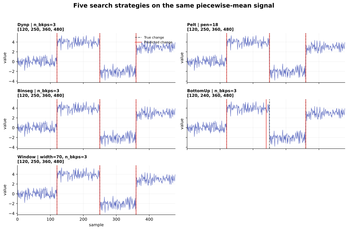
The signal has four constant-mean regions and true breakpoints [120, 250, 360, 480]. The five detectors share the same L2 segment cost, but they search for a partition differently.

Detector	Stopping rule	Prediction
Dynp	exactly 3 changes	[120, 250, 360, 480]
Pelt	penalty 18.0 per change	[120, 250, 360, 480]
Binseg	exactly 3 changes	[120, 250, 360, 480]
BottomUp	merge until 3 changes remain	[120, 240, 360, 480]
Window	select 3 local discrepancy peaks	[120, 250, 360, 480]

Dynp evaluates the fixed-number objective exactly on the candidate grid. Pelt instead lets a penalty decide how many changes are worth keeping. The other three are approximate search strategies. On this particular signal, BottomUp places one change at sample 240 rather than 250 because its early local merges constrain the later answer. That visible difference is useful: sharing a cost does not make the search algorithms equivalent.

import rustures as rpt

dynp = rpt.Dynp(model="l2", min_size=20, jump=2)
pelt = rpt.Pelt(model="l2", min_size=20, jump=2)

fixed_k = dynp.fit_predict(signal, n_bkps=3)
penalized = pelt.fit_predict(signal, pen=18.0)

Three views of the same two-feature signal

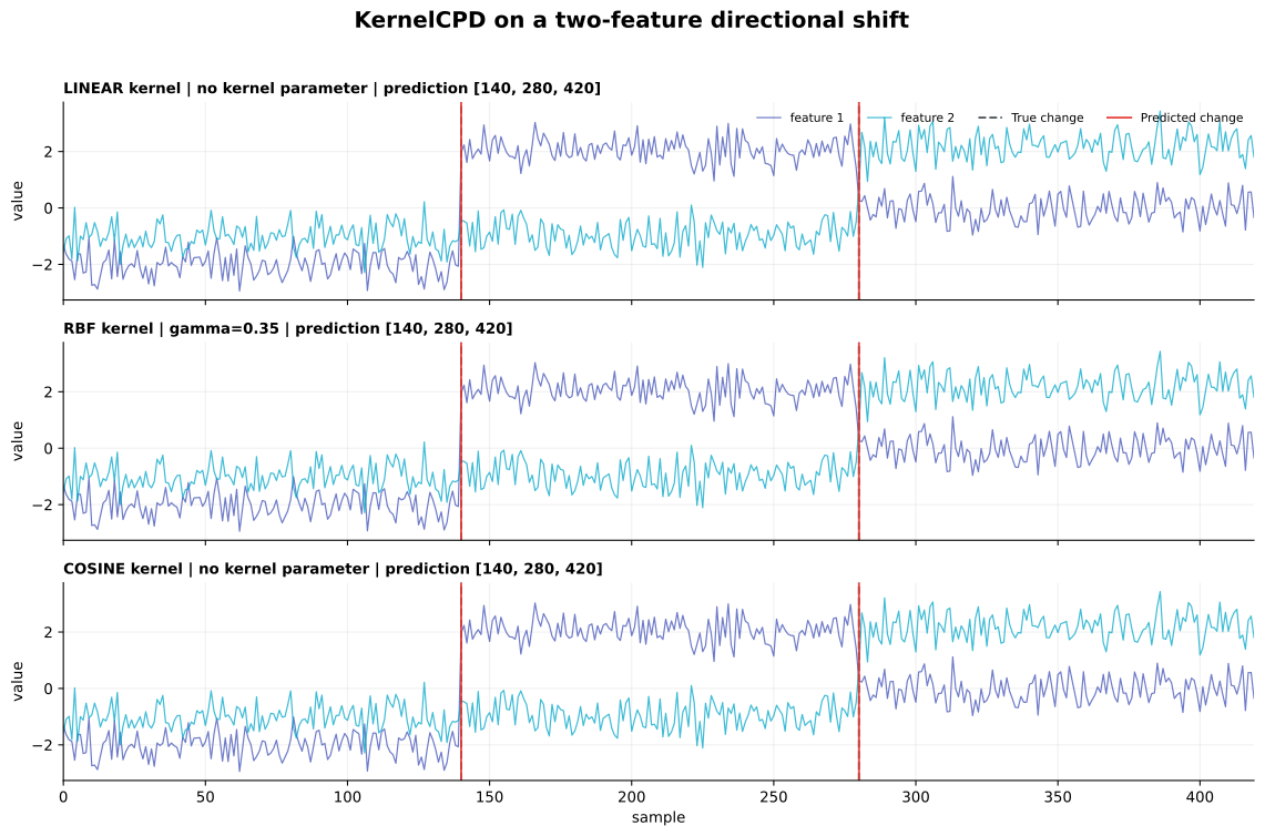
Here every observation has two features. The underlying two-dimensional center changes at samples 140 and 280. Each feature contributes to the kernel similarity; KernelCPD does not segment the feature columns independently.

Kernel	Parameters	Prediction
Linear	fused backend	[140, 280, 420]
RBF	fused backend, gamma=0.35	[140, 280, 420]
Cosine	fused backend	[140, 280, 420]

All three kernels recover these deliberately clear center shifts. This does not mean the kernels are interchangeable. Linear similarity emphasizes changes in ordinary feature space, RBF similarity can expose nonlinear distribution changes, and cosine similarity emphasizes direction while reducing sensitivity to magnitude. See Costs and kernels for the objective behind these choices.

prediction = rpt.KernelCPD(
    kernel="rbf",
    gamma=0.35,
    backend="fused",
    min_size=20,
    jump=2,
).fit_predict(signal_2d, n_bkps=2)

Outliers and robust objectives

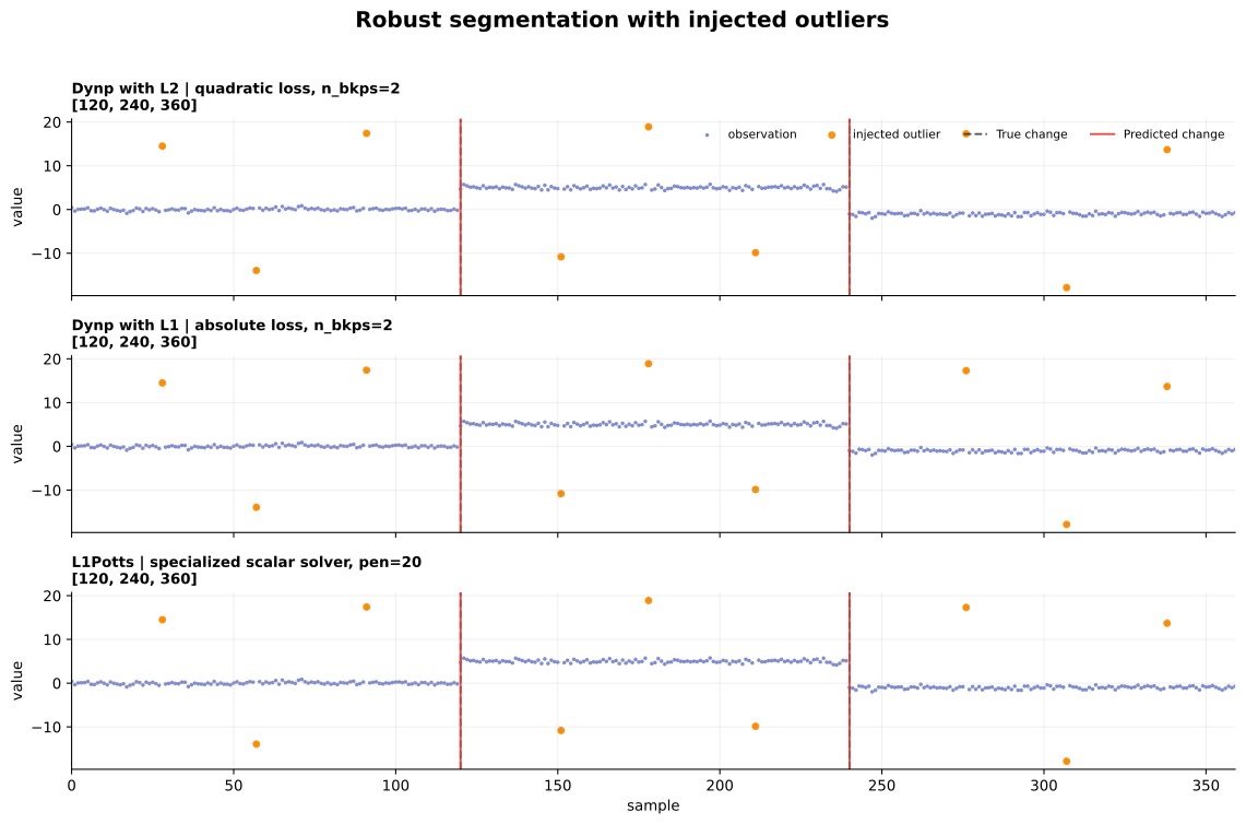
The orange points are nine deliberately injected outliers. The known piecewise median changes at samples 120 and 240.

Method	Objective	Prediction
Dynp(model="l2")	fixed 2 changes, squared deviations	[120, 240, 360]
Dynp(model="l1")	fixed 2 changes, absolute deviations	[120, 240, 360]
L1Potts	penalized scalar L1-Potts, pen=20.0	[120, 240, 360]

All three succeed on this sample, but for different reasons. L2 fits a mean and squares residuals, so a large outlier has disproportionate influence. L1 fits a median and grows only linearly with the residual size. L1Potts combines that robust scalar loss with its own specialized penalized solver, whereas Dynp solves a general fixed-number partition problem. A single successful plot is not a robustness guarantee; it makes the different objectives concrete.

fixed_two = rpt.Dynp(model="l1", min_size=20).fit_predict(
    scalar_signal,
    n_bkps=2,
)
automatic_count = rpt.L1Potts().fit_predict(scalar_signal, pen=20.0)

Reproduce every figure

The charts are generated by the committed figure-generation script, not hand-edited. Install a release wheel plus NumPy and Matplotlib, then run:

python -m pip install rustures numpy matplotlib
python scripts/generate_docs_figures.py

The exact seeds, parameters, and returned lists are also stored in machine-readable result metadata. Generated SVGs are committed so GitHub Pages does not need to compile Rustures or install Matplotlib.

Complete notebooks

The repository also contains two executable Jupyter tutorials:

• English tutorial
• Korean tutorial

GitHub renders both notebooks in the browser. To execute one locally, clone the repository and install Jupyter with Rustures.

git clone https://github.com/denrew88/rustures.git
cd rustures

python -m venv .venv
python -m pip install --upgrade pip
python -m pip install rustures jupyter matplotlib
python -m jupyter lab

Activate .venv first if your shell does not automatically use it.

More minimal recipes

Fixed number of mean changes

signal, truth = rpt.pw_constant(
    n_samples=500,
    n_features=2,
    n_bkps=3,
    noise_std=0.5,
    seed=42,
)

prediction = rpt.Dynp(model="l2", min_size=10, jump=1).fit_predict(
    signal,
    n_bkps=3,
)

Unknown number of changes

prediction = rpt.Pelt(model="l2", min_size=10, jump=1).fit_predict(
    signal,
    pen=12.0,
)

Custom Bernoulli likelihood

See Custom Python costs for the full protocol and a vectorized implementation pattern. The same approach works for Poisson counts, categorical likelihoods, weighted domain losses, and other additive interval objectives.

Reproducible synthetic data

Rustures includes deterministic generators:

rpt.pw_constant(...)
rpt.pw_linear(...)
rpt.pw_normal(...)
rpt.pw_wavy(...)

Every generator returns (signal, breakpoints) and accepts an explicit seed. A seed is reproducible within a Rustures version; generated streams may change across versions when the implementation is optimized.